Imagine you move to a new street and want to guess how much your house is worth. A sensible shortcut: find the five houses nearest to yours and look at their sale prices. No spreadsheets, no formulas, just “what did the people around me do?”
That instinct is the entire idea behind K-Nearest Neighbours (KNN). To classify a new data point, KNN looks at the K closest points to it in the training data and lets them vote. Want to guess if someone will like a new coffee shop? Find the K people most similar to them (in taste, spending habits, location) and go with the majority opinion. No model is trained in advance, no assumptions about the shape of the data. You just ask the neighbours.
It is popular because it is simple, requires almost no setup, and works surprisingly well when similar things really do behave similarly. The catch is a single number you have to choose yourself: K, the number of neighbours to consult.
How KNN actually draws the line
The plot below shows KNN in action on a simple two-class problem (blue vs orange).
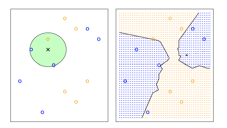
On the left, the black x is a new observation. KNN draws a circle just big enough to capture its three nearest neighbours (here, mostly blue), and assigns the majority class. Do this for every point in the space and you get the jagged black boundary on the right, the line that separates “KNN says blue” from “KNN says orange”.
The problem: what is the right K?
Small K means each prediction is based on just a handful of very close neighbours, so the boundary above would twist and turn to chase every last data point. Large K means the boundary gets averaged over many neighbours and becomes smoother, but less sensitive to local detail. This trade-off shows up clearly when you plot error rate against model flexibility.
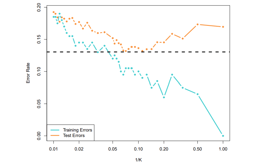
The x-axis here is 1/K, so moving right means K is shrinking and the model is getting more flexible. The blue training error keeps falling, and if you push K all the way down to 1, it hits zero: the model just memorises every training point as its own nearest neighbour. That looks like a win, but it is not, because training error is not what we actually care about. What matters is the orange line: how well the model performs on data it has never seen.
And the orange line does not cooperate. It falls for a while alongside the training error, then turns around and climbs back up. Past a certain point, extra flexibility stops capturing real signal and starts fitting noise, quirks specific to the training set that will not repeat in new data. That is overfitting, and it is exactly what the shrinking gap between the two lines on the right-hand side of the plot is showing you.
Go too far the other way (K very large, 1/K near zero) and the model swings toward underfitting. Every prediction gets smoothed over such a large neighbourhood that real group differences get washed out, and the model becomes too biased to draw meaningful boundaries between classes at all.
The sweet spot sits at the bottom of the orange U, marked by the dashed line. Somewhere in the middle, not so small that the model reacts to noise, not so large that it goes blind to real structure. That balance point, between variance on one side and bias on the other, is the entire job when tuning K.
The lesson generalises well beyond KNN: a model that keeps getting better on training data is not necessarily getting better at its actual job. Always check the test error before you believe the training error.